
Great Curves Deserve Quadratic Regression
Speaking of the Simplex Method, I’ll definitely be writing a future article about that algorithm. We gotta warm up to it though, so we’ll start by stretching out our brains with some quadratic regression. Remember that previous article I wrote about the transformation of a function? Back by popular demand, it’s Sketch A!
(where y = x-squared)
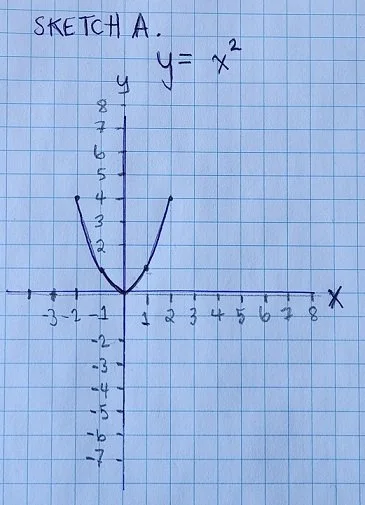
In Sketch A. we express y as a function of x, where x is squared:
f(x) = x * x
We didn’t really delve into all the rules that apply whenever the term “function“ is used. We won’t be discussing those rules in this article, but don’t worry we’ll get to them!
For now, we’re going to add a little more to our x-squared expression: another (non-squared) x, and a plain, old constant value. What’s a “constant value“? A constant value stays the same regardless of what else is happening in an equation. In our expression, the value of x will change but our constant value stays the same. It looks like this:
y = (x*x) + x + constant value
Remember that x*x is very different from x+x, so we’ve got to keep those two expressions separate even though each x has the same value. Because the x-value is subject to change, we call it a “variable“. This means the letter ‘x‘ is a placeholder for a value that changes. The letter ‘y‘ is also a placeholder, and its value is dependent on whatever value we put into our x-variable.
Is there anywhere else we can put some constant values? We could put a constant value in front of each x:
y = constant(x*x) + constant(x) + constant
The only problem with this is it appears as though the value of each constant is the same, and that may not be the case. What if each constant value is different? To account for this possibility, we’ll give each constant value a separate name. We’ll call the first constant value ‘a‘, the second constant ‘b‘, and the third ‘c‘:
y = a(x*x) + b(x) + c
Our curvy function just got a little fancier, so we’ll give it a fancier name to match: quadratic equation. Whenever you see an expression where a variable is multiplied by itself at least once (x-squared), know that you’re looking at a quadratic function. There’s also a fancy name for the shape of this curve: parabola. When the first term (the ‘a‘) in our quadratic function is positive, the parabola is a smile. If that first term is negative, then the parabola is a frown.
QUADRATIC REGRESSION
You might be wondering, what’s the point of all this? Why did we bother making our curve so fancy, and where’s the regression part of this quadratic stuff? Well, quadratic expressions help us to represent curves that are a little more subtle than x-squared. There are a lot of peaks and valleys out there that just don’t fit into something as simple as an x-squared. We’re surrounded by them every day, including the increase and decrease of the temperature wherever you are. When the sun rises, so does the temperature. At some point during the day, the temperature reaches its highest point and then starts to decrease. This may happen multiple times a day, but we’re going to look at one temperature peak and see if we can predict when it will start to decrease.
Personally, I’m not too fond of hot weather. For example if the temperature at noon is 24.67 degrees Celsius, and 25.0 degrees at 1:00pm, then 25.22 degrees at 2:00pm, I wanna know, “Hey! When’s it going to start cooling down?“ Lets see if we can use these three temperatures (or data points) to make that prediction. It’s time for a new
SKETCH B!
I’ll admit, these three data points don’t give us much of a curve, however they’re all we need to calculate the model that will help us predict when the temperature will start to decrease. The values for a, b, and c give us a mathematical model that we can apply to a later time in the day, or a different value of x. Furthermore, the c-value in our quadratic equation always matches the y-intercept. That gives us one more piece of data to help make a prediction:
y = a(x*x) + b(x) + 24.67
Remember, the y-intercept is where x equals zero, or in this case, noon. All we’re missing now are the two different values ‘a‘ and ‘b‘ that we must multiply by x-squared and x.
OBTAINING THE MATHEMATICAL MODEL
If you can’t stand the suspense, I’ll give you a short-cut: it’s called the “Omni Calculator”. It’s a great online resource that you can use to obtain the mathematical model for a quadratic function, given at least three data points. If you want, you can use it to verify the model we’re about to obtain. Since we already know that where x equals zero our y-value equals 24.67, we’ll move on to our second data point: (1, 25).
25 = a(1*1) + b(1) + 24.67
We subtract 24.67 from both sides of the equation, and we’ll put the x-value in front of ‘a’ and ‘b’:
25 - 24.67 = 1a + 1b, which becomes
0.33 = a + b
We’ll stop there for a moment, and move on to our last data point: (2, 25.22)
25.22 = a(2*2) + b(2) + 24.67, becomes
25.22 - 24.67 = 4a + 2b
We’ll pull a ‘2‘ out of the right side of this equation, so we can apply it to the left side:
0.55 = 2(2a + b)
This is called ‘factoring’, and Khan Academy does a great job of explaining the operation in more detail. Here, we’ll use it to further simplify both sides of our equation (dividing by 2):
0.55/2 = 2a + b, which gives us
0.275 = 2a + b
We’ll stop again because we’ve got two expressions that we can put together to obtain a value for ‘a‘ or ‘b‘. From our second data point above, we can obtain a value for ‘b‘ in terms of ‘a‘:
0.33 - a = b
We can substitute that expression into ‘b‘ for our other data point:
0.275 = 2a + (0.33 - a), becomes 0.275 = 2a + 0.33 - a
then
0.275 - 0.33 = 2a - a
-0.055 = a
That’s a good sign! Literally!
We know that our parabola is shaped like a frown, so we’re expecting our ‘a‘ term to be negative. Lets try substituting our value for ‘a‘ to get a value for ‘b‘:
0.33 - (-0.055) = b
0.385 = b
MAKING THE PREDICTION
We’ve got our mathematical model!!
y = -0.055(x*x) + 0.385x + 24.67
Now we can make a prediction for x=3, and x=4.
y = -0.055(3*3) + 0.385(3) + 24.67
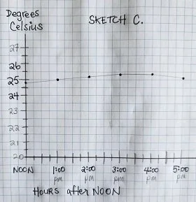
SKETCH C. shows a temperature plateau from 3:00 to 4:00pm
Unfortunately for me, if the temperature decreases at the same rate that it increased then it won’t start to get cooler until at least 5:00pm. According to our mathematical model, the temperature will reach a high of 25.33 between 3:00 to 4:00pm. By 6:00pm the temperature should return to 25 degrees. So 2:00 Christine better start making some ice cubes and settle in the shade with a nice cool drink, cuz it’s gonna be a long, warm day!